The numerical corner-transfer matrices (CTM) method is a powerful variational algorithm suitable for studying 2D and 3D systems in statistical mechanics and quantum physics. With some modifications it can be also used for investigating properties of 1D and 2D quantum systems.
Our recent results for the scaling function of the 2D Ising model in a magnetic field obtained using the CTM method are available:
Here we describe square lattice variant of variational CTM method with one binary degree of freedom (i.e. spin) at each lattice vertex and a combination of four such spins (plaquette) as building block of the lattice (this is called IRF - Interaction Round Face model).
Usual method of solving such statistical model is breaking the lattice into infinite stripes, considering one stripe as a matrix of probabilities of having particular configuration at each stripe boundary. Such a matrix is called Transfer Matrix(TM), and it was introduced by Kramers and Wannier[4]. For numerical approximation lattice on a cylinder is used, and TM becomes finite. Usually one looks for largest eigenvalues of TM, since the largest one represents equilibrium state (thus gives partition function) and the next ones give slightly excited states.

But there is a major problem of TM in numerical solution of finite lattices. Adding one more site to the lattice doubles (for Ising case) the size of TM. Since near the critical point correlation leghth is big, we need lots of sites to get reasonably accurate answers. Since it's currently impossible to handle matrices larger than 2N where N>20÷25, extrapolation by N or other similar methods are used thus accuracy decreases greatly.
Another problem with row-to-row TM is its spectrum. Next-to-ground state of TM is highly degenerate, degree of degeneracy is generally proportional to the size of the system. Gap width between ground state and highly degenerate next-to-ground states is proportional to distance to the critical point. This further complicates handling of TM for systems near critical point.
So, in many cases using Corner Transfer Matrix (CTM) could give significant advantange over Kramers-Wannier Transfer Matrix.
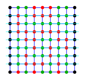
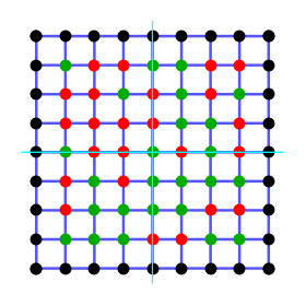
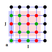
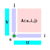
Now let's consider square lattice again and cut into four pieces (instead of stipes) as shown below:
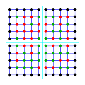
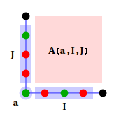
Each of the four parts of the lattice can be represented as a (infinite) matrix with matrix indexes enumerating states on both cuts. Such matrix is called Corner Transfer Matrix (CTM) of the model.
Note that for all non-zero matrix elements spin at the corner must be the same for both sides of the matrix; alternatively, representation where a is just a separate variable can be used.
As it was said above, CTM spectrum falls much faster than spectrum of ordinary TM, e.g. degeneracy of level next to ground state is small number fixed in respect to CTM size and proportional to the size of the system for TM. Thus similar sizes of both CTM and TM lead to much better accuracy for CTM methods.
Since we consider an infinite lattice, these many equivalent partitions are, Lattice partition shown above is not unique in respect of defining the CTM, we might leave one or several rows along the cuts. Half-infinite row, called Half-Row Matrix (HRTM) will be used below.
After multiplying all weights inside quater of the lattice and somehow normalizing resulting matrix one can forget about internal structure. Usual normalization is division by highest eigenvalue.
One should note, that, in principle, reducing from infinite to finite CTM doesn't correspond to reducing infinite lattice to finite sublattice. Indeed, infinite lattice can be described by CTM in appropriate basis very well, much better than by TM of the same size.
For symmetric lattice A is symmetric too. So in priciple we can choose basis where A matices are diagonal. This is the case for the most practical calculations, because of intentional truncation of CTM spectrum.
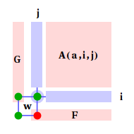
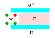
Thus, after taking into account all weights away from the boundaries, and, after a basis change, whole lattice is represented as:

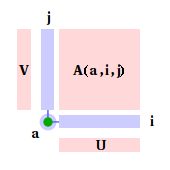
where matrices U and V are diagonalization matrices, V=UT for symmetric A.
Note, that corner spin was exlcuded from transformation and left in the natutal basis.
In practice, direct minimization (e.g. using Newton method) of κ(A,F) functional seems to be not very useful approach, since dimension of space of possible variations is quite high. Nishino and Okunishi proposed the very physically-sensible iteration procedure, which has very good convergence even in the vicinity of critical point.
First step of iteration is building lattice extended by one face by multiplying CTM with two half-row F matrices and one Boltzmann weight. Resulting matrix is a CTM too, but it's non-diagonal, although still symmetic. Obviously, it has double size in respect to original CTM.
Then one diagonalizes this CTM (for non-symmetic case similar procedure, e.g. SVD, is used) and get diagonal CTM A' with eigenvalues sorted in descending order and its diagonalization (i.e. basis-changing) matrix. For general iteration then the half of matrix with smaller eigenvalues is dropped, giving the matrix of original size. In diagonalized matrix half of the rows are also dropped, so it become "basis-changing and projecting" matrix.
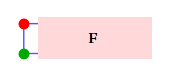
Now one should proceed to HRTMs, thus change their basis too. First, one extends HRTM by attaching a Boltzmann weight to the side of HRTM. Then we take diagonalization-projection matrices, obtained from CTMs and and multiply the exended HRTM by them.
Initial state for this iteration scheme can be chosen in different ways. It can be small matrices representing "frozen" state, or one can use full-sized matrices corresponding to the finite piece of the lattice and build of exact Boltzmann weights.
